Using RAM in Offshore Wind Project Series - Design Phase

Offshore Wind's Decade of Transformation
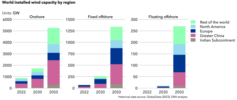
The global offshore wind industry has seen remarkable growth. By the end of 2022, a total of 66 GW of offshore wind capacity was operational across three continents and 19 countries, accounting for 7% of global wind power installations. This is more than 12 times the installed capacity compared to 20121. More importantly, the technology is now more cost competitive and is shifting to other parts of the world. In North America and Asia, for example, there are ambitious plans for very large-scale offshore wind generation capacity as shown in Figure 1. A major factor in the acceleration of these developments is the radical cost reduction of offshore wind energy, particularly in the last five years.
One of the key drivers in the growth of offshore wind is due to location. Offshore locations typically offer a more dependable and higher velocity wind resource than onshore sites, resulting in relatively more consistent and reliable energy output, thereby rendering offshore wind farms notably more efficient in electricity generation when compared to their land-based counterparts. Moreover, one of the key benefits of offshore wind farms is they do not take up valuable land coastal space, allowing potential multifaceted use of coastal areas2. Lastly, the expanse of offshore environments facilitates the deployment of larger and more robust wind turbines, unhindered by the spatial constraints often encountered on land. Higher capacity turbines mean that fewer turbines are needed to generate the same amount of energy across a wind farm —ultimately leading to lower costs. Offshore wind farms undoubtedly have the potential to generate far more energy than onshore alternatives, but this enhanced output comes with higher capital and maintenance costs that requires careful consideration.
Challenges to Offshore Wind
Despite the recent steady growth of the offshore wind turbines (OWTs), their development lags that of onshore turbines due to the high cost of power production associated with OWTs. As of 2022, wind power contributed 7% to global grid-connected electricity output. The lion's share of this was from onshore wind farms, while a mere 0.6% was attributed to fixed offshore wind1. This is largely due to the higher levelized cost of energy (LCOE) for OWTs, which represents the average life-cycle price of the electricity generated from a given power source per megawatt-hour, is employed to compare different power sources. On a global average, the LCOE for onshore wind is estimated at USD 49/MWh, whereas for offshore wind, it stands at USD 80/MWh1.
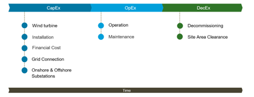
LCOE consists of various components, including but not limited to Capital Expenditure (CAPEX), Operations and Maintenance (O&M), financing costs, permitting costs, it is observed in most cases CAPEX is a significant of the total cost of the wind farm project over its entire lifespan. CAPEX encompasses expenses related to turbine, substructures (platform, mooring and anchoring), and transmission system (cables and substations). Given that CAPEX often represents the highest proportion of the LCOE for wind projects, it is crucial for owners to strategize effectively to reduce costs at the early stages of development as well as total lifetime expenditure.
Additionally, availability for onshore wind turbines is generally reported to be between 95% and 97% for modern systems4. This is facilitated by easy accessibility which allows frequent maintenance on these turbines. For OWTs face additional challenges due to the location and the associated difficulties in accessing the site and the harsher weather conditions, which can lead to an unacceptable down time level. This makes it inevitable to assess the O&M demand of an offshore wind farm in conjunction with the other design parameters to achieve the required availability level against optimal cost expenditure. The latter being a tradeoff between investment costs to increase the reliability and the cost of maintenance actions to boost the availability to a high level. Since site accessibility always has a level below 100% for offshore conditions, it is paramount to focus on optimizing the overall asset performance of OWTs.
In this article, we will delve into how owners can address these challenges by achieving the optimal balance between financial considerations and asset availability through the application of Reliability, Availability, and Maintainability (RAM) methodology.
RAM Approach to Tackling Design and Engineering Challenges
Reliability, Availability and Maintainability (RAM) analysis is a methodology used to predict asset performance based on reliability and maintainability. This methodology is well established and used in many domains such as the oil and gas and transport industries, and increasingly in the renewables industry.
With wind turbine capacity, equipment reliability, dynamic feed and demand, maintenance constraints, weather conditions, supply chain issues, etc., it’s nearly impossible to calculate the impact of one change to a system — because all these factors are highly interrelated, and one change can start a chain reaction of events. To simulate all these interconnected uncertainties, DNV’s RAM tools Maros and Taro applies Monte Carlo simulation technique, which is based on repeated random sampling to obtain numerical results. This assigns random values to model variables – for example, process downtimes and equipment repair times in probabilistic manner. The use of dynamic simulation techniques allows estimations taking account of continuous changes in the state of the system over its expected life. RAM considers the uncertainty inherent in complex systems such as in an offshore wind farm, it can provide alternative approaches compared to deterministic analysis in which fixed values are used for model variables.
RAM analysis is typically used to predict the performance of wide range of energy systems and to provide a basis for the optimization of such systems. The nature of it will vary according to the purpose of the study and the scope of work. However, in many cases, RAM analysis is used to predict system availability and identify ways to improve system availability by considering both equipment failures and maintenance factors. To illustrate the benefits of RAM (reliability, availability, maintainability) analysis for wind farm project in engineering phase, let's delve into a case study that demonstrates its value in real-world scenarios.
Offshore Wind Farm Case Study – Reliability
The offshore wind farm consists of 10 wind turbine generators, each with a 2MW installed capacity, giving the farm an aggregate 20MW installed capacity. The base case model consists of both the wind turbines and Offshore Substation (OSS) with the following considerations:
- All wind turbine systems have similar components.
- Some clusters consistently receive high wind speeds, while others receive lower wind speeds.
- The tower and sub-structure of the wind turbines are not included in the model.
- Corrective Maintenance (CM) will be carried out whenever a fault is detected on first-come, first-served basis.
When performing a RAM study, a Block Flow Diagram (BFD) defines the connectivity of nodes and focuses on the generation aspects of the system e.g. wind profiles. Each node within the network will require its own Reliability Block Diagrams (RBDs). Reliability Block Diagrams (RBDs) are used to outline the logical relationships between the different events. Each one of the blocks in a Reliability Block Diagram represents one “event” that can lead to generation loss. RBDs are a logical representation of the system connection considering path of success of the system mission, in this case electricity generation. If items are configured in series, when one of them is in a failed state there is no way for the system to move forward. However, if you have items in parallel, it means that there more than one “success” path in the system.
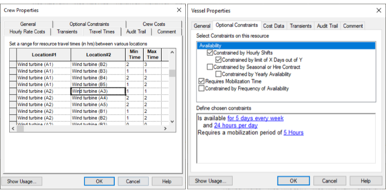
Once we know what equipment items to be included in the model, we start looking into collecting reliability data. Typically, these data could be sourced from industry data, vendor data or in-house data. Commonly used failure and repair distributions supported in DNV’s Maros and Taro includes Exponential, Weibull, Normal, Log-Normal, Triangular, Rectangular etc.
Offshore Wind Farm Case Study – Maintainability
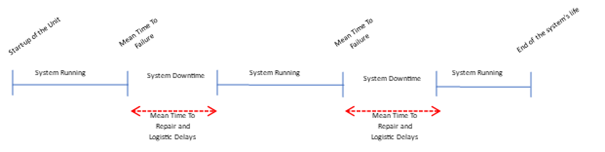
Maintenance is a critical element in the LCOE, given the practical constraints imposed by offshore operations and the relatively high costs. The selection of maintenance strategies influences the overall efficiency, profit margin, safety, and sustainability of offshore wind farms. Consider a generic event, a failure, or a planned shutdown. In real life, this failure will start being repaired with a certain delay time corresponding to the time required to diagnose the problem and organize the repair resources to carry out necessary repairs. Once all resources are on the job location, the actual repair procedure can commence. The repair action itself may impact the generation capabilities in another manner. Therefore, maintenance resources must be accounted for when performing a RAM study for wind farm projects.
At design and engineering phase, high level details on the maintenance requirements can be obtained from the vendor or past experiences. Modelling maintenance logistics involves determining the ‘repair delay’ portion of the above sequence. This is achieved by defining the location, quantity and constraints of the various resources involved in the repair process. Simulation is then carried out to determine each repair delay depending upon the foregoing and the workload at the instant of the failure. It is not simply a case of specifying a repair delay per task. It is important to understand how these logistics manifest themselves in the simulation.
This case study considers great level of detail regarding maintenance strategy – remember offshore wind farm is unmanned and remote so it is requiring special type of maintenance strategy. Incorporating the maintainability aspects will increase the quality of the outputs of the RAM analysis.
Offshore Wind Farm Case Study – Availability
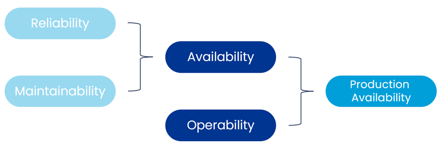
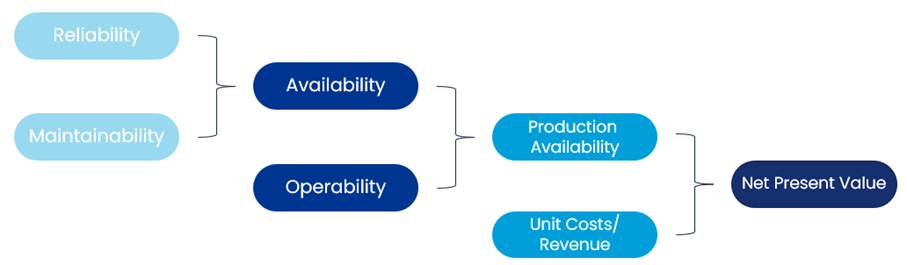
By combining both reliability and maintainability, one would get the availability. This is the ratio between the time a wind farm is operational and the total time it could have been operational. It reflects how reliably the wind farm can operate and produce electricity when needed.

Time-based availability, while important, offers only a partial view of a wind farm's performance. It measures the operational uptime of turbines but overlooks the critical factor of energy output. For example, wind speeds can vary significantly over time. A wind turbine may be highly available during periods of low wind, but its output and therefore its contribution to overall energy production might be minimal.
Offshore Wind Farm Case Study – Production Availability
To better assess a wind farm's performance, DNV’s Maros and Taro considers production availability – units of achieved generation in kWh or MWh. This metric measures the amount of energy produced relative to the potential energy that could have been produced, considering the variability of wind resources and the performance of the turbines. To obtain production availability, we add operability - wind profile, restart time, recovery mechanisms etc. By incorporating production availability, wind farm operators can gain accurate understanding of the efficiency and productivity of their wind farm, enabling them to identify areas for improvement and optimization.
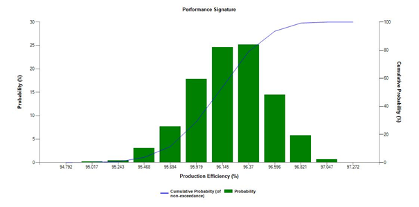
The virtual model for the wind turbine simulates 12500 cycles. This means the model is sampling events for 500 different lives of 25 years. The calculated production availability for the system is 96.098% with a standard deviation of 0.331%. This production availability is averaged from all the simulated lifecycles. A graph showing the distribution of the different production availability throughout the different lifecycles can be generated.
From this graph, the analyst can assess the probability of different levels of generation. Traditionally, engineers are interested on the P10 and P90 probabilities for a system. In this case study, we can see that 10% of the estimated production availability lifecycle will not exceed 95.675% and 90% of the estimated production availability lifecycle will not exceed 96.514%.
In addition, as we are tracking the impact of equipment failures on generation, we get a criticality list which is a ranking of all equipment items/systems and the average generation loss caused by these items. The criticality breakdown and ranking identify system “weak points” or “bad actors” and ranks the equipment items and systems (and other events if applicable) by their contribution to the production availability losses. This allows us to quickly see the largest contributors to generation losses and focus our efforts on improving the performance of these major contributors to downtime.
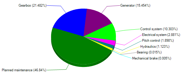
For this model, the biggest contributors for the generation loss are:
- The “Planned Maintenance” is responsible for 46.84% of the losses.
- The “Gearbox system” is responsible for 21.48% of the losses.
- The “Generator system” is responsible for 15.45% of the losses.
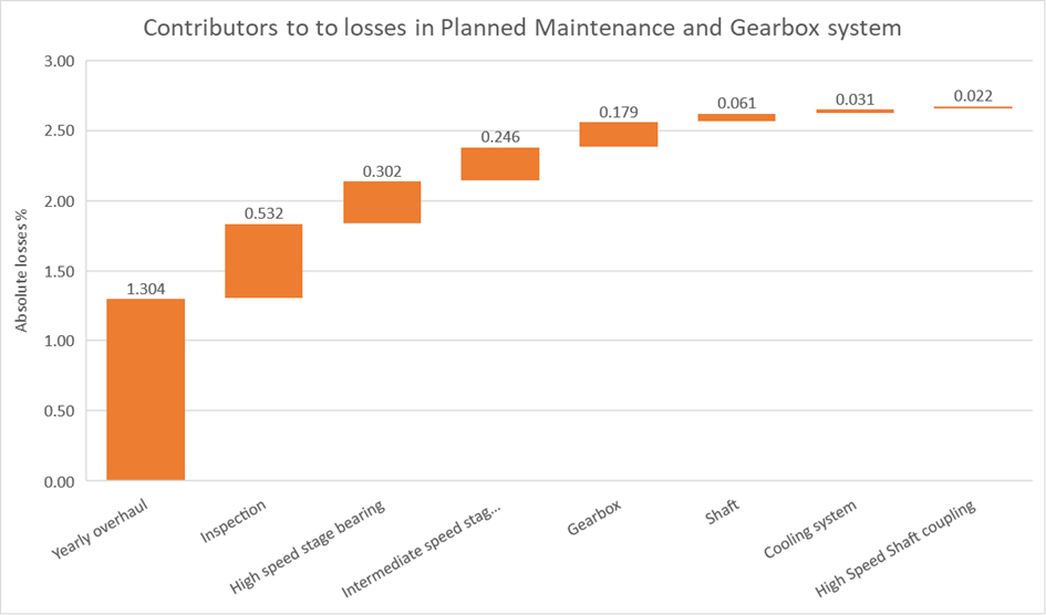
The major contributors to losses can be further investigated. The planned maintenance is expected and the ability to quantify how much generation is lost due to planned shutdowns is important. However, generation loss can also be tracked for the unscheduled outages such as the second biggest contributor, the Gearbox.
Armed with the information regarding the subsystem criticality, the analyst can incorporate the costs and revenues from the project and subsequently investigate different changes to the design or maintenance strategy. This gives guidance on the mitigation effort on optimizing the system. Once one design scenario has been tested, it can be accepted or not depending on the return on performance.
Offshore Wind Farm Case Study – Net Present Value
To compliment the decision-making process, it is crucial to strike a balance between optimizing availability and cost-effectiveness. While having the best availability through high redundancy and reliability might seem appealing, it can lead to increased costs that may not be justifiable in the long run. A well-rounded financial assessment should weigh the benefits of increased availability against the associated costs, ensuring that the project remains economically viable and efficient.
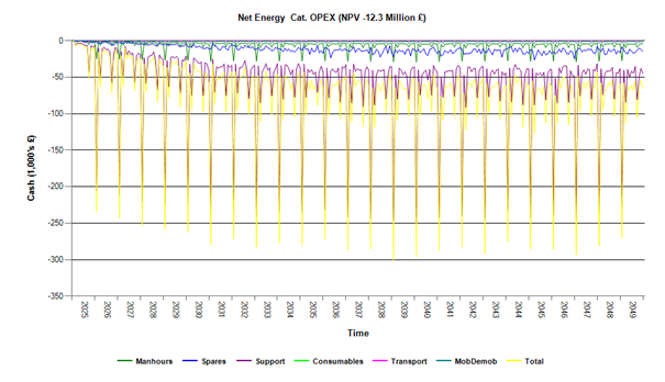
A view of the financial aspects of the venture can also be evaluated looking at the cash flow, operational expenditure, and cumulative revenue. The graph below shows the lost generation recovery opportunity. Thus -£12.3M shows how much money we can recover if we can optimize the system to avoid generation loss. When assessing the opportunity costs associated with a project, stakeholders need to consider the potential revenue that could be generated if the project operates at optimal levels. This is where RAM analysis becomes essential. By evaluating the reliability and availability of the assets, stakeholders can identify potential bottlenecks, inefficiencies, or areas of improvement that, if addressed, could lead to significant cost savings and increased revenue.
For example, a RAM analysis can help stakeholders understand the impact of equipment downtime on generation and revenue. By analyzing the data, they can determine the optimal maintenance strategies, spare parts inventory, and equipment redundancy to minimize downtime and maximize generation. This, in turn, can help them make informed decisions about investments in equipment upgrades, maintenance practices, and operational procedures, ultimately leading to reduced operational expenditure and increased cumulative revenue.
Moreover, a RAM analysis can also help stakeholders identify and quantify the potential financial benefits of implementing improvements. By comparing the current state of the assets with the projected improvements, stakeholders can estimate the potential savings in terms of reduced maintenance costs, increased generation capacity, and improved operational efficiency. This information can then be used to prioritize investments and allocate resources effectively, ensuring that the organization maximizes its return on investment.
Wrapping it up…
RAM analysis plays a key role when analyzing optional combinations of design configuration, maintenance strategy and operational rules, in the oil and gas industry. Informed decisions can be made and uncertainty regarding the generation behavior can be accurately predicted and therefore avoided or reduced.
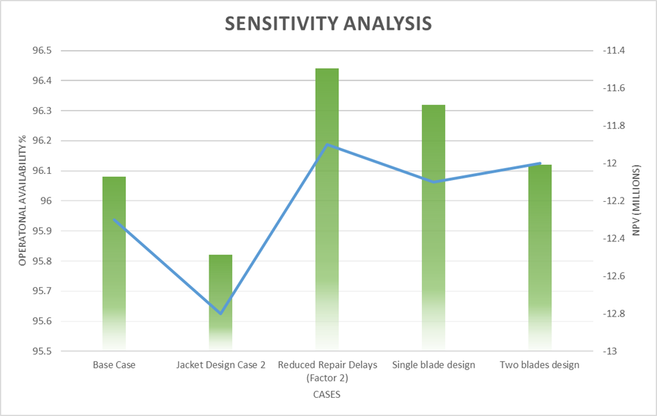
A list of possible design options can be created from a base case. These options can then be ranked showing the effectiveness and financial benefits of each one of them.
How DNV can help
Grounded in our expertise in technical and regulatory aspects, DNV supports owners in realizing wind projects in a safe and cost-efficient manner. We have the technical expertise that enabled us to work on 97% of the world’s offshore wind projects. With a deep understanding of the entire offshore wind system, DNV helps stakeholders to mature offshore wind concepts from the idea to implementation. And the great thing is coupled with advisory insights and wide range of software solution, DNV’s RAM tools Maros and Taro can be applied to help provide faster and more accurate decision-making in striking a balance between reliability enhancement and minimizing downtime-related productivity losses. With technology that gives you an up-close look at the entire system and models the effects of changing conditions throughout, you can decide what adjustments to make with complete confidence and maximize your return on investment.